Machine Learning with Scikit Learn: knn and log classification

Introduction

Setup

library(reticulate)
library(here)

here() starts at /home/joao/JR-IA

py_discover_config()

python:         /home/joao/JR-IA/renv/python/condaenvs/renv-python/bin/python
libpython:      /home/joao/JR-IA/renv/python/condaenvs/renv-python/lib/libpython3.7m.so
pythonhome:     /home/joao/JR-IA/renv/python/condaenvs/renv-python:/home/joao/JR-IA/renv/python/condaenvs/renv-python
version:        3.7.13 (default, Mar 29 2022, 02:18:16)  [GCC 7.5.0]
numpy:          /home/joao/JR-IA/renv/python/condaenvs/renv-python/lib/python3.7/site-packages/numpy
numpy_version:  1.21.6

NOTE: Python version was forced by RETICULATE_PYTHON

import numpy as np
import pandas as pd
import matplotlib.pyplot as plt
import seaborn as sns
from sklearn.model_selection import train_test_split
from sklearn.neighbors import KNeighborsClassifier
from sklearn.metrics import confusion_matrix, classification_report
from sklearn.linear_model import LogisticRegression
from sklearn.metrics import roc_curve
from sklearn.metrics import roc_auc_score

Data load and transform

#diabetes_df = pd.read_csv("posts/20230113/data/diabetes_clean.csv")

diabetes_df = pd.read_csv("data/diabetes_clean.csv")
X = diabetes_df.drop("diabetes", axis=1).values
y = diabetes_df["diabetes"].values
X_train, X_test, y_train, y_test = train_test_split(X, y, test_size=0.4, random_state=42)

KNN classification

Fit, Predict

knn = KNeighborsClassifier(n_neighbors=6)
knn.fit(X_train, y_train)

KNeighborsClassifier(n_neighbors=6)

y_pred = knn.predict(X_test)

Metrics

print(confusion_matrix(y_test, y_pred))

[[176  30]
 [ 56  46]]

print(classification_report(y_test, y_pred))

              precision    recall  f1-score   support

           0       0.76      0.85      0.80       206
           1       0.61      0.45      0.52       102

    accuracy                           0.72       308
   macro avg       0.68      0.65      0.66       308
weighted avg       0.71      0.72      0.71       308

The report produces metrics for the two cases we may want to use the model too: predict the persons who don’t have diabetes (0) or predict persons with diabetes (1). In the first case for example the precision is 0.75.

Logistic regression

Fit, Predict

logreg = LogisticRegression()
logreg.fit(X_train, y_train)

LogisticRegression()

/home/joao/JR-IA/renv/python/condaenvs/renv-python/lib/python3.7/site-packages/sklearn/linear_model/_logistic.py:765: ConvergenceWarning: lbfgs failed to converge (status=1):
STOP: TOTAL NO. of ITERATIONS REACHED LIMIT.

Increase the number of iterations (max_iter) or scale the data as shown in:
    https://scikit-learn.org/stable/modules/preprocessing.html
Please also refer to the documentation for alternative solver options:
    https://scikit-learn.org/stable/modules/linear_model.html#logistic-regression
  extra_warning_msg=_LOGISTIC_SOLVER_CONVERGENCE_MSG)

y_pred = logreg.predict(X_test)
y_pred_probs = logreg.predict_proba(X_test)[:, 1]
print(y_pred_probs[:10])

[0.2947024  0.19804295 0.14437254 0.1691528  0.51158775 0.4799649
 0.01555761 0.60402434 0.53766079 0.78702341]

ROC

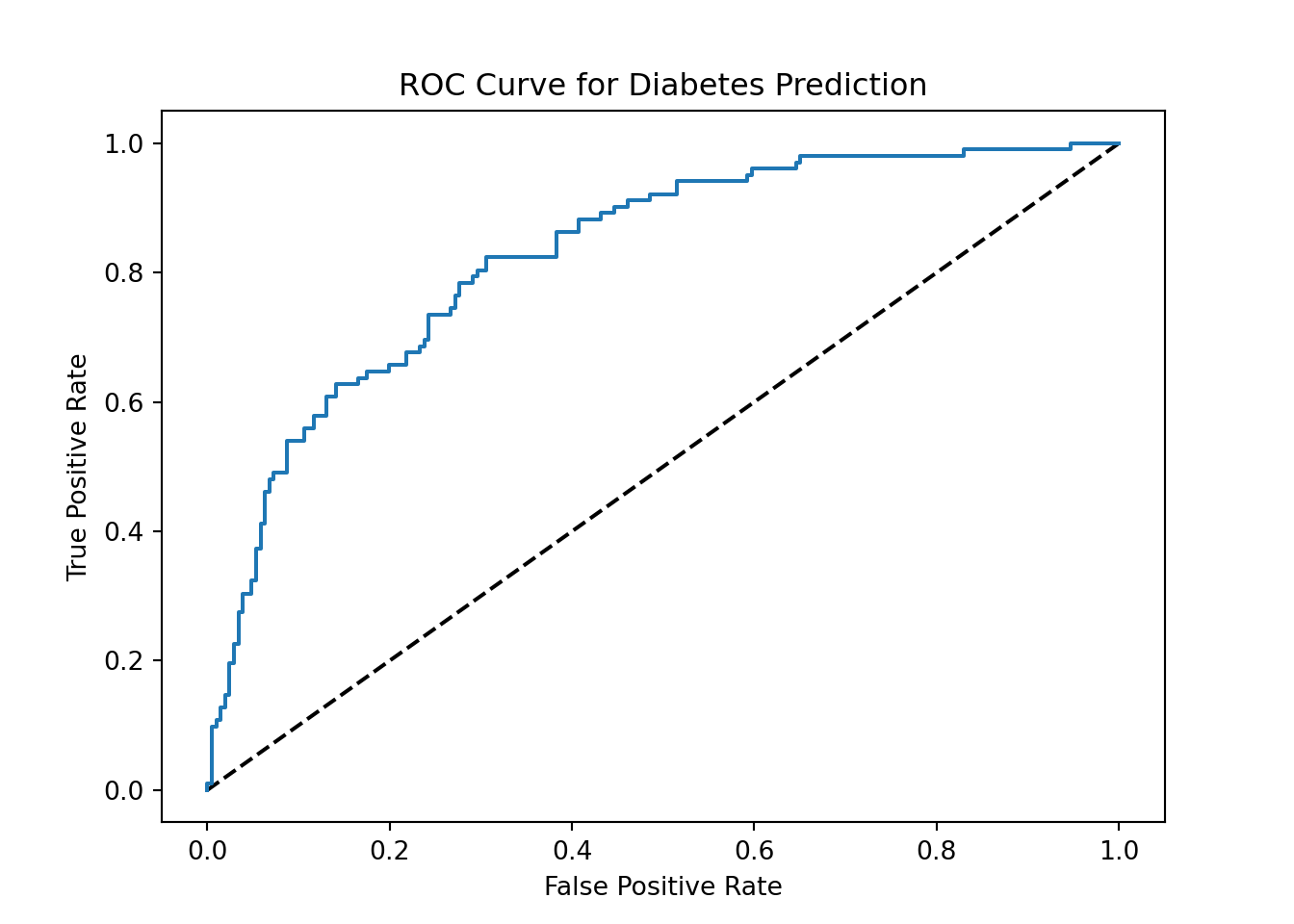
fpr, tpr, thresholds = roc_curve(y_test, y_pred_probs)
print("ROC AUC:", roc_auc_score(y_test, y_pred_probs).round(4))

ROC AUC: 0.8261

plt.clf()
plt.plot([0, 1], [0, 1], 'k--')
plt.plot(fpr, tpr)
plt.xlabel('False Positive Rate')
plt.ylabel('True Positive Rate')
plt.title('ROC Curve for Diabetes Prediction')
plt.show()

Metrics

print(confusion_matrix(y_test, y_pred))

[[170  36]
 [ 36  66]]

print(classification_report(y_test, y_pred))

              precision    recall  f1-score   support

           0       0.83      0.83      0.83       206
           1       0.65      0.65      0.65       102

    accuracy                           0.77       308
   macro avg       0.74      0.74      0.74       308
weighted avg       0.77      0.77      0.77       308

Memo

Formulas

• accuracy: ( tp + tn ) / tt
• precision: tp / ( tp + fp )
• sensitivity: tp / ( tp + fn )
• f1 score: 2 * precision * sensitivity / (precision+sensitivity)

Labels

• tp: true positives
• tn: true negatives
• fp: false positives
• fn: false negatives
• tt: total

Definitions

• accuracy: the proportion of the data that are predicted correctly

• precision: high precision means low false positives

• recall (sensitivity): high sensitivity means low false negative

• f1 score:

• KAP (kappa): similar to accuracy, but normalized by the accuracy that would be expected by chance alone

• LogLoss: alternative to MSE and MAE (compared with accuracy, the logarithmic loss takes into account the uncertainty in the prediction)

• ROC auc: area under the receiver operator curve

• specificity: of only the truly negative, what proportion is classified as negative

• overlap: the proportion of times the model fails in predicting correctly