Machine Learning with Scikit Learn: linear regression

machine learning

Author

João Ramalho

Published

December 17, 2022

Introduction

This posts initiates a new series on Machine Learning with Python. Previous posts have focused on Machine Learning with R using the tidymodels framework. This new series follows the same kind of modelling workflow from data loading, feature engineering, modelling, predicting new values and evaluating model performance.

The main objectives of these posts is to serve as a cookbook for Machine Learning and be a complement of my book ‘industRial data science’ released in 2021 that doesn’t cover predictive.

Setup

My favorite configuration for Data Science has stabilized in RStudio with Quarto and the Reticulate package. In previous posts I have shown comparisons of different commercial software, programming languages and programming tools and IDEs. This RStudio-Quarto-Reticulate covers all use cases I can imagine both for professionals and non-professionals with the smallest configuration effort possible (still there is some!).

library(reticulate)
library(here)

here() starts at /home/joao/JR-IA

py_discover_config()

python:         /home/joao/JR-IA/renv/python/condaenvs/renv-python/bin/python
libpython:      /home/joao/JR-IA/renv/python/condaenvs/renv-python/lib/libpython3.7m.so
pythonhome:     /home/joao/JR-IA/renv/python/condaenvs/renv-python:/home/joao/JR-IA/renv/python/condaenvs/renv-python
version:        3.7.13 (default, Mar 29 2022, 02:18:16)  [GCC 7.5.0]
numpy:          /home/joao/JR-IA/renv/python/condaenvs/renv-python/lib/python3.7/site-packages/numpy
numpy_version:  1.21.6

NOTE: Python version was forced by RETICULATE_PYTHON

Checking the path during workbook rendering

print(paste0("here() path: ", here()))

[1] "here() path: /home/joao/JR-IA"

print(paste0("R path: ", getwd()))

[1] "R path: /home/joao/JR-IA/posts/20221217"

import os
print("Python path:", os.getcwd())

Python path: /home/joao/JR-IA/posts/20221217

condaenv = here("renv/python/condaenvs/renv-python")
reticulate::conda_install("scikit-learn", envname = condaenv)

import numpy as np
import pandas as pd
import matplotlib.pyplot as plt
import seaborn as sns
from sklearn.linear_model import LinearRegression
from sklearn.model_selection import train_test_split
from sklearn.metrics import mean_squared_error
from sklearn.model_selection import cross_val_score, KFold

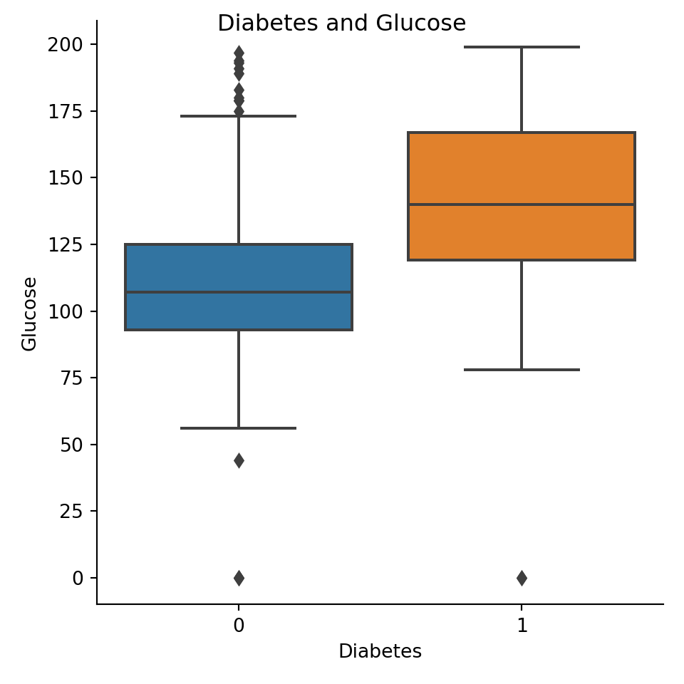
Data load

This example is based on the Data Camp course on Supervised Learning with Scikit learn. The dataset is quite interesting with several variables and close to 1000 datapoints. Although it is small from a machine learning point of view it is big enough for demonstration purposes.

#diabetes_df = pd.read_csv("./posts/20221217/data/diabetes_clean.csv")
diabetes_df = pd.read_csv("data/diabetes_clean.csv")

print(diabetes_df.shape)

(768, 9)

print(diabetes_df.columns)

Index(['pregnancies', 'glucose', 'diastolic', 'triceps', 'insulin', 'bmi',
       'dpf', 'age', 'diabetes'],
      dtype='object')

print(diabetes_df.head())

   pregnancies  glucose  diastolic  triceps  ...   bmi    dpf  age  diabetes
0            6      148         72       35  ...  33.6  0.627   50         1
1            1       85         66       29  ...  26.6  0.351   31         0
2            8      183         64        0  ...  23.3  0.672   32         1
3            1       89         66       23  ...  28.1  0.167   21         0
4            0      137         40       35  ...  43.1  2.288   33         1

[5 rows x 9 columns]

Data transform

As usual in Scikit learn models we have first to convert the dataframe to pandas arrays and separate inputs from outputs. This is heavier that in R where dataframes are kept together but there is certainly a speed trade off on the long term.

X = diabetes_df.drop("glucose", axis=1).values
y = diabetes_df["glucose"].values

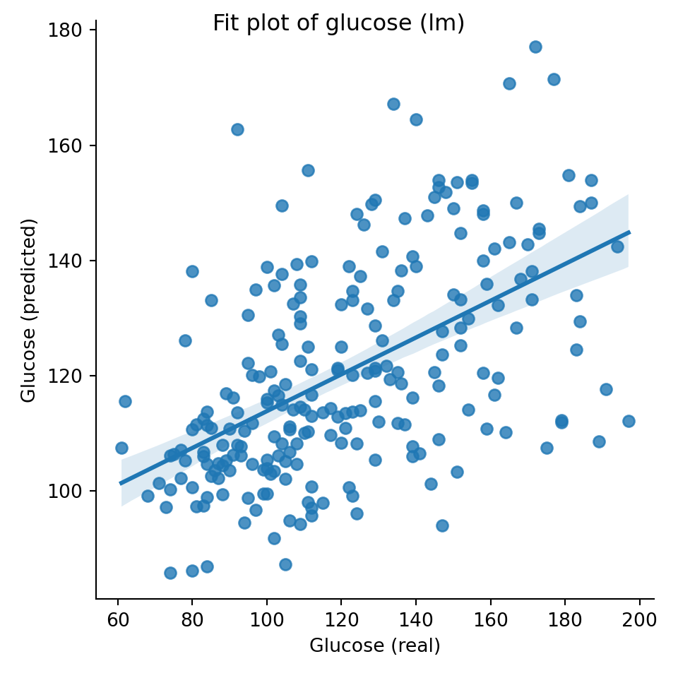
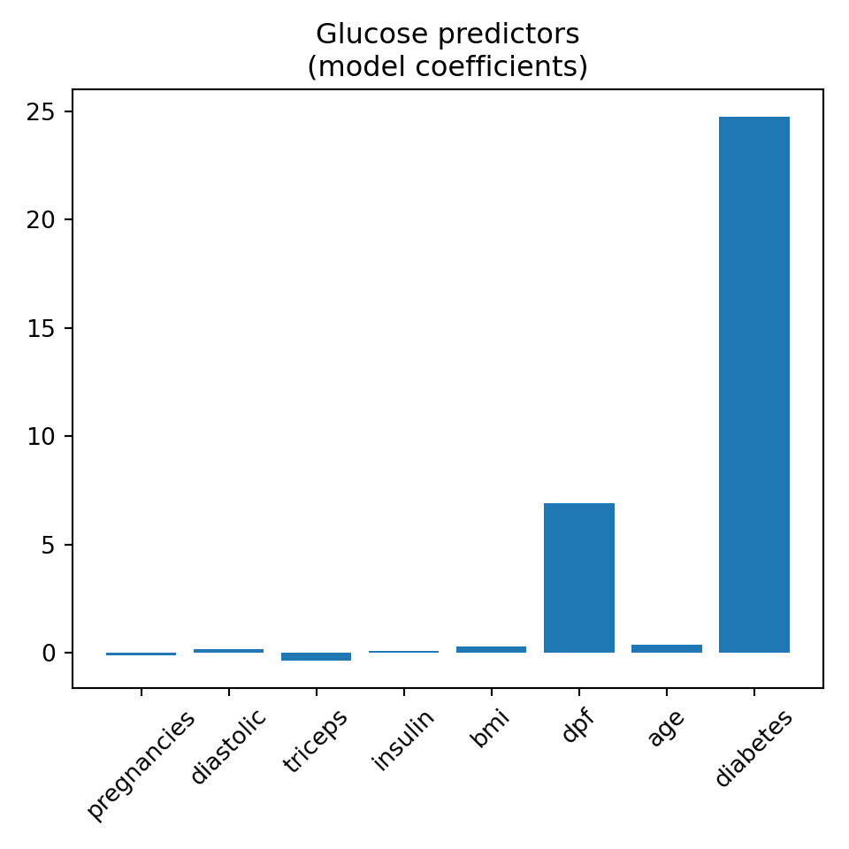
Multiple linear regression

We observe that in general the syntax is simpler than in R tidymodels and the workflow can be complete in just a few lines.

Split

X_train, X_test, y_train, y_test = train_test_split(X, y, test_size=0.3, random_state=42)

Fit

reg_all = LinearRegression()
reg_all.fit(X_train, y_train)

LinearRegression()

Predict

y_pred = reg_all.predict(X_test)

Metrics

reg_all.score(X_test, y_test)

0.28280468810375103

mean_squared_error(y_test, y_pred, squared=False)

26.341459582232265

Fit plot

print(y_test.shape, y_pred.shape)

(231,) (231,)

dict_lmplot = {'y_test' : y_test, 'y_pred' : y_pred}
data_lmplot = pd.DataFrame(data=dict_lmplot)

plt.clf()
g = sns.lmplot(x = 'y_test', y = 'y_pred', data = data_lmplot)
g.set(xlabel="Glucose (real)", ylabel="Glucose (predicted)")

g.fig.suptitle("Fit plot of glucose (lm)")
plt.tight_layout()
plt.show()

Coeficients

names = diabetes_df.drop("glucose", axis=1).columns
coefs = reg_all.coef_
print(reg_all.intercept_)

77.3665487857505

VI plot

plt.clf()
plt.bar(names, coefs)

<BarContainer object of 8 artists>

plt.title("Glucose predictors\n(model coefficients)")
plt.xticks(rotation=45)

([0, 1, 2, 3, 4, 5, 6, 7], <a list of 8 Text major ticklabel objects>)

plt.tight_layout()
plt.show()

In this example we see that diabetes is a strong predictor of glucose.

Confirm with R

Having R as a primary language I’m confirming here below for learning purposes that the same results are obtained with the lm function.

diabetes_r <- py$diabetes_df
model_glucose <- lm(glucose ~ ., diabetes_r)
broom::tidy(model_glucose) |> 
  knitr::kable(digits = 2)

term	estimate	std.error	statistic	p.value
(Intercept)	77.80	5.20	14.97	0.00
pregnancies	-0.47	0.34	-1.38	0.17
diastolic	0.12	0.05	2.23	0.03
triceps	-0.29	0.07	-4.03	0.00
insulin	0.09	0.01	9.81	0.00
bmi	0.31	0.14	2.21	0.03
dpf	1.69	2.95	0.57	0.57
age	0.48	0.10	4.87	0.00
diabetes	25.04	2.18	11.49	0.00

X-y plot

plt.clf()
g = sns.catplot(x = 'diabetes', 
                y = 'glucose', 
                kind = 'box',
                #capsize = 0.1,
                data = diabetes_df)
g.set(xlabel="Diabetes", ylabel="Glucose")

g.fig.suptitle("Diabetes and Glucose")
plt.tight_layout()
plt.show()

Cross validation

kf = KFold(n_splits=6, shuffle=True, random_state=5)
reg = LinearRegression()
cv_scores = cross_val_score(reg, X, y, cv=kf)

print(cv_scores)

[0.37915966 0.29257178 0.38953015 0.22314647 0.3677666  0.31175482]

print(np.mean(cv_scores))

0.3273215793495467

print(np.std(cv_scores))

0.058445441569060494

print(np.quantile(cv_scores, [0.025, 0.975]))

[0.23182464 0.38823384]