Authoring with Quarto: jupyter python template workbook

tools

Published

August 4, 2022

Objective

This article serves as a template for Python using a jupyter notebook that is rendered in a quarto site. It uses a conda installation that has been configured previously (see article from the 2022-04-09). The conda environment needs to be indicated in the notebook configuration for the cells to run. The conda environment needs to be activated in the bash terminal before rendering the website.

Introduction

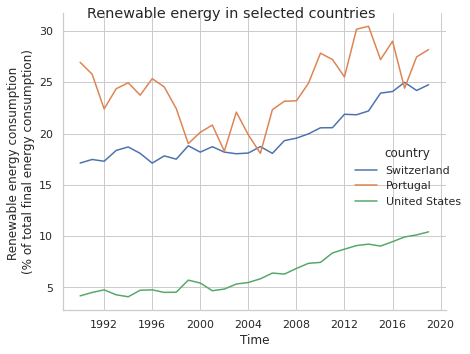
In this article we’re exploring another open data source, this time the World Bank. The topic selected for testing the data collection and visualization is the share of renewable energy for selected countries in the last 25 years. The article also confirms the compatibility of the python programming language in this website which is build with the R programming language.

Setup

%conda env list

Install wbdata

The World Bank website suggests several methods to obtain the data from its databases. After some reading we’ve opted here for the python module wbdata. The possibilities to install the module are described in wbdata documentation. In our website the python configuration has been done with conda which is not available. We’ve then opted for a direct download from github and saved the library folder directly in our project folder. This has been enough to make it available. The chunk below confirms that python sees the module.

We can then import it in a python chunk directly as below:

import wbdata

Dependencies install

When trying to run the module in our setup, several dependencies were missing. We keep the code here of the installation for future reference.

Load modules

Besides loading wbdata we also need to load the common python libraries for data wrangling and plotting:

import pandas as pd
import matplotlib.pyplot as plt
import seaborn as sns
import datetime
import json

Now we’re ready for data loading and exploration.

Renewable electricity output

Search country by code

As in similar articles we’ve opted to call the API as least as possible and to store the data objects locally. This avoids loading the entity servers and ultimately to see one’s access blocked. Our starting point has been the selection of countries for our analysis. The wbdata API provides a method to get countries called get_country. In the next chunk we show how we have queried once the data base for all the countries and save it as a json object.

renewables_country_list=wbdata.get_country()
with open('data/renewables_country_list.json', 'w') as json_file:
  json.dump(renewables_country_list, json_file)

Now we can load anytime we like from our local folder:

with open('data/renewables_country_list.json', 'r') as json_file:
  country_list = json.load(json_file)

The returned object is a list of dictionaries. We can check the entry for Switzerland with:

country_list[47]

{'id': 'CHE',
 'iso2Code': 'CH',
 'name': 'Switzerland',
 'region': {'id': 'ECS', 'iso2code': 'Z7', 'value': 'Europe & Central Asia'},
 'adminregion': {'id': '', 'iso2code': '', 'value': ''},
 'incomeLevel': {'id': 'HIC', 'iso2code': 'XD', 'value': 'High income'},
 'lendingType': {'id': 'LNX', 'iso2code': 'XX', 'value': 'Not classified'},
 'capitalCity': 'Bern',
 'longitude': '7.44821',
 'latitude': '46.948'}

Later in our query for renewable energy we will only need the country id. It can be obtained from the list by sub setting as follows:

country_list[47]['id']

'CHE'

To extract all countries codes we can run a for loop as follows:

country_codes = []
for i in range(0,len(country_list)):
  country_id = country_list[i]['id']
  country_codes.append(country_id)

print(country_codes[0:9])

['ABW', 'AFE', 'AFG', 'AFR', 'AFW', 'AGO', 'ALB', 'AND', 'ARB']

This was a possible approach but it requires knowing the countries codes upfront. In case they’re not know there’s another country search method that accepts various arguments the search_countries method shown below.

Search country by name

We’re using here the keyword argument to provide country names. We start by creating a list with the country names that we feed in the loop. Using a similar sub setting approach with the index [0] and then the [‘id’] we can extract the code and assign it to a list.

target_countries = ['United States', 'Portugal', 'Switzerland']

country_codes = []
for country in target_countries:
  country_entry = wbdata.search_countries(country)
  country_code = country_entry[0]['id']
  country_codes.append(country_code)

print(country_codes)

This country_codes list is the one that we will use later in our query for renewable energy figures.

Search indicators

Now that our countries are selected we’re going to identify an indicator of interest on which to make the analysis. As before we do this only once and store the result to a json object.

#indicators_list = wbdata.search_indicators('renewable energy')
#with open('data/renewables_indicators_list.json', 'w') as json_file:
#  json.dump(indicators_list, json_file)

Now for the purposes of analysis and investigation we reload the indicators object as often as we need:

with open('data/renewables_indicators_list.json', 'r') as json_file:
  indicators_list = json.load(json_file)

For the sake of testing we’re exploring here a different way of looking into the json file. Less intuitive but easier than the for loop is to use the pandas method json_normalize:

indicators = pd.json_normalize(indicators_list)
indicators[['id', 'name']]

Using this information we prepare the variable for the final query. In this case it is sufficient to do it manually.

indicators = {'EG.FEC.RNEW.ZS':'renewable_energy_perc_total'}

Get data

There are various methods to get the data from the world bank database. Again there is a json approach and one directly with pandas. As we have only one indicator and three countries we’re opting for a simpler approach with pandas. This should be sufficient as we don’t expect deeply nested data which is one of the main benefits of the json format.

We query the database once and store the result in a local csv file.

#renewables=wbdata.get_dataframe(indicators, country = country_codes, convert_date = True)
#renewables.to_csv("data/renewables.csv")

NameError: name 'indicators' is not defined

We load it for our analysis:

renewables=pd.read_csv("data/renewables.csv")
print(renewables.head())

       country        date  renewable_energy_perc_total
0  Switzerland  2021-01-01                          NaN
1  Switzerland  2020-01-01                          NaN
2  Switzerland  2019-01-01                        24.76
3  Switzerland  2018-01-01                        24.20
4  Switzerland  2017-01-01                        24.99

Although not strictly needed for seaborn we’re removing the missing values, which we consider to be a good general practice:

renewables.dropna(axis=0,subset=['renewable_energy_perc_total'], inplace=True)
print(renewables.head(5))

       country        date  renewable_energy_perc_total
2  Switzerland  2019-01-01                        24.76
3  Switzerland  2018-01-01                        24.20
4  Switzerland  2017-01-01                        24.99
5  Switzerland  2016-01-01                        24.10
6  Switzerland  2015-01-01                        23.94

And a final step is to convert the date to the datetime format which will open several possibilities and ensure a much better looking plot:

renewables['date'].dtype
renewables['date'] = pd.to_datetime(renewables['date'], infer_datetime_format=True)
renewables['date'].dtype

dtype('<M8[ns]')

Plot

We’ve opted to use seaborn. In particular when we want to use the hue this is a good approach. We assign the plot to a variable to allow to call directly some matplotlib methods for axis configuration:

sns.set_theme(style="whitegrid")
g=sns.relplot(x='date', y='renewable_energy_perc_total', hue='country', data=renewables, kind='line')
g.set(xlabel = 'Time', ylabel = 'Renewable energy consumption \n(% of total final energy consumption)')
g.fig.suptitle('Renewable energy in selected countries')
plt.tight_layout()
plt.show()