Eurostats: GDP per capita

econometrics

Published

April 26, 2022

A comparison of the GDP per capita from 2000 to 2020, in 6 representative EU countries

We’ve introduced Eurostats in our article from early February this year when we looked into unemployment and we went into some detail on how to get data from this important open data repository. Now in this article we’re analysing GDP per capita across several countries spanning from lowest to highest income to get a general view of unemployment in Europe.

As we’re using the R programming language, we start by loading some libraries we will need for the analysis:

knitr::opts_chunk$set(comment = NA)
library(here)
library(eurostat)
library(readr)
library(dplyr)
library(forcats)
library(ggplot2)

Data

We’ve made previously a search in the Eurostat database and identified the table sdg_08_10 as having the data we need.

In order to avoid connecting to the Eurostat everytime we run our code, we made a local copy with the code below:

sdg_08_10 <- get_eurostat("sdg_08_10")
write_csv(sdg_08_10, here("posts/20220426/data/sdg_08_10.csv"))

We can now load it directly from our data folder:

data_raw <- read_csv(here("posts/20220426/data/sdg_08_10.csv"))

Rows: 1681 Columns: 5
── Column specification ────────────────────────────────────────────────────────
Delimiter: ","
chr  (3): unit, na_item, geo
dbl  (1): values
date (1): time

ℹ Use `spec()` to retrieve the full column specification for this data.
ℹ Specify the column types or set `show_col_types = FALSE` to quiet this message.

The previous output from read_csv shows that our dataset has 1681 entries but only 5 variables. It also indicates also their name and type. Looking into the time variable we see our dataset spans the last 20 years aproximately:

min(data_raw$time); max(data_raw$time)

[1] "2000-01-01"

[1] "2021-01-01"

unique(data_raw$na_item)

[1] "B1GQ"

A unique “na_item” is available. Looking into the site instructions we see this corresponds to the Gross domestic product at market prices

unique(data_raw$unit)

[1] "CLV10_EUR_HAB"   "CLV_PCH_PRE_HAB"

Again the site provides explanations for the two unit types, these are:

Chain linked volumes (2010), euro per capita [CLV10_EUR_HAB]
Chain linked volumes, percentage change on previous period, per capita [CLV_PCH_PRE_HAB]

We’ll retain absolute values for our analysis. The dataset also provides various countries which we can see with:

unique(data_raw$geo)

 [1] "AL"        "AT"        "BE"        "BG"        "CH"        "CY"       
 [7] "CZ"        "DE"        "DK"        "EA19"      "EE"        "EL"       
[13] "ES"        "EU27_2020" "EU28"      "FI"        "FR"        "HR"       
[19] "HU"        "IE"        "IS"        "IT"        "LT"        "LU"       
[25] "LV"        "MK"        "MT"        "NL"        "NO"        "PL"       
[31] "PT"        "RO"        "RS"        "SE"        "SI"        "SK"       
[37] "TR"        "UK"        "ME"

We’re selecting 6 countries trying to sample the bottom, top and the middle of the income rank.

country_list <- c("PT", "LU", "CH", "PL", "RO", "DE")

We now apply our filters on unit and country to our dataset:

data_short_CLV10_EUR_HAB <- data_raw |>
    filter(unit == "CLV10_EUR_HAB") |>
    filter(geo %in% country_list)

Conviniently the eurostats R package provides also a labeling function which is very useful. To obtain labels we pass our dataset to the function with some specific arguments. Again we’ve made a local copy of the labelled dataset, now using the code below:

sdg_08_10_CLV10_EUR_HAB_labelled <- label_eurostat(
    data_short_CLV10_EUR_HAB, 
    custom_dic = c(DE = "Germany"), 
    lang = "en") |>
    mutate(geo = fct_relevel(
        geo, c("Luxembourg", "Switzerland", "Germany", "Portugal", 
               "Poland", "Romania")))

write_csv(sdg_08_10_CLV10_EUR_HAB_labelled, here("posts/20220426/data/sdg_08_10_CLV10_EUR_HAB_labelled.csv"))

And we’re here loading the labeled dataset:

sdg_08_10_CLV10_EUR_HAB_labelled <- read_csv(here(
  "posts/20220426/data/sdg_08_10_CLV10_EUR_HAB_labelled.csv"), 
  show_col_types = FALSE) |> 
      mutate(geo = fct_relevel(
        geo, c("Luxembourg", "Switzerland", "Portugal", "Poland", "Romania"))) |> 
  filter(geo != "Germany") |> 
  filter(time >= lubridate::as_date("2009-01-01"))


sdg_08_10_CLV10_EUR_HAB_labelled[sample(3),1:3]

# A tibble: 3 × 3
  unit                                         na_item                     geo  
  <chr>                                        <chr>                       <fct>
1 Chain linked volumes (2010), euro per capita Gross domestic product at … Pola…
2 Chain linked volumes (2010), euro per capita Gross domestic product at … Swit…
3 Chain linked volumes (2010), euro per capita Gross domestic product at … Luxe…

Taking here 3 rows at random from the table, we can see that the units, na_item and geo entries have been replaced by some more understandable labels.

Plot

Having sourced, filtered and labeled the data we are now ready to generate a plot:

sdg_08_10_CLV10_EUR_HAB_labelled |>
    mutate(geo = fct_relevel(geo, c("Luxembourg", "Switzerland", "Portugal", "Poland", "Romania"))) |> 
    ggplot(aes(x = time, y = values, color = geo)) +
    geom_line() +
    scale_y_continuous(
        n.breaks = 10, 
        name = "Euro", labels = scales::label_number()) +
    scale_color_brewer(palette = "Set1", name = "Country") +
    theme_light() +
    labs(
        title = "GDP per Capita",
        subtitle = "Gross Domestic Product at Market Prices",
        caption = "Source: Eurostats sdg_08_10"
    )

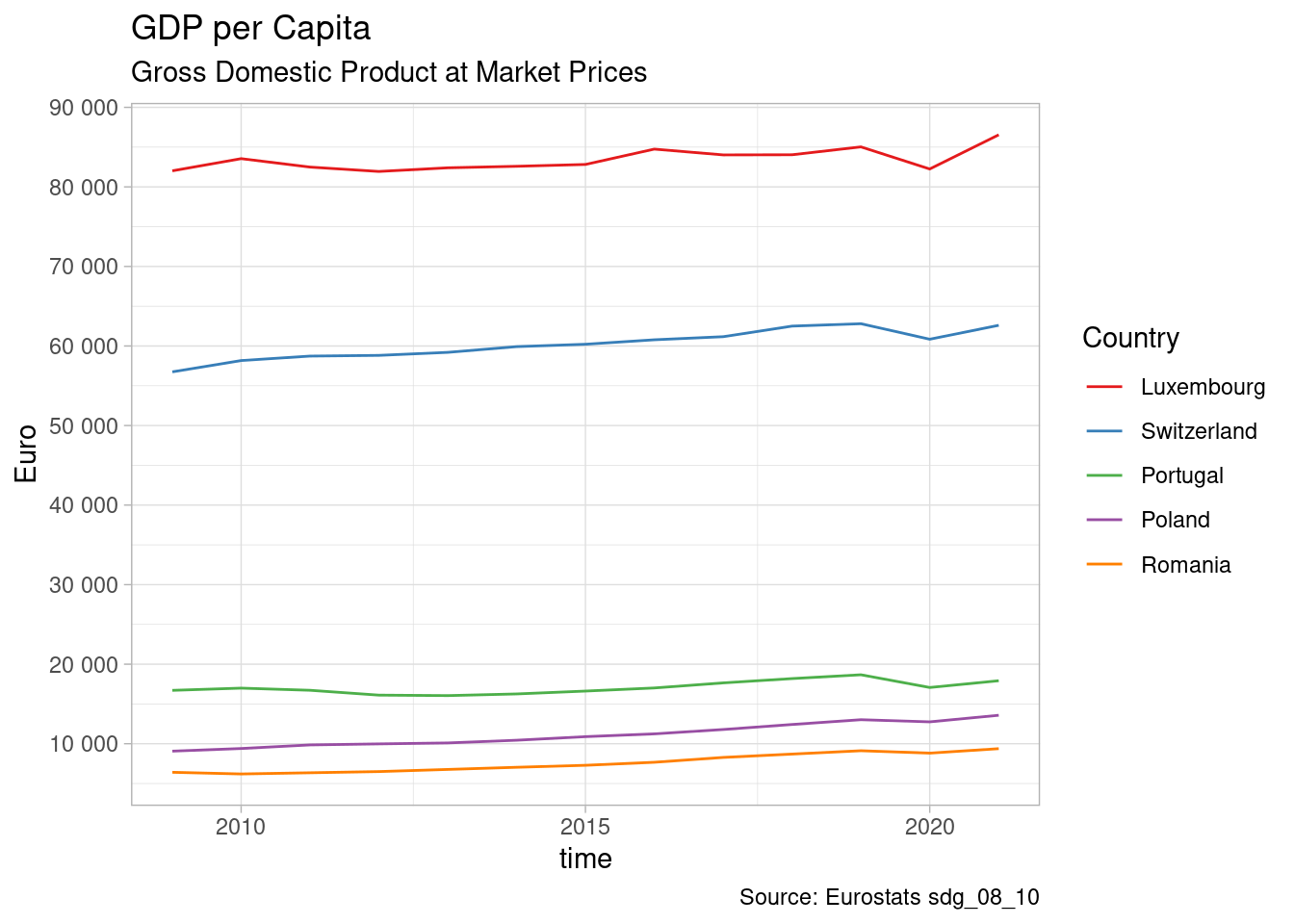
In the plot we see that GDP per capita varies immensely inside the EU ranging from Eur 10’000 to Eur 90’000. GDP per capita has progressing in the last 20 years in spite of two major crise. We can also see that countries that had the highest income are also the ones with the highest growth.