Eurostats: knowledge employement

econometrics

Published

February 12, 2022

Progress of knowledge intensive employment in Europe since 2009

Open data is key for governments, for policy making but also for citizens to form a view. Public statistics have been publicly available since long but now with open data and moderately accessible data tools it is possible to get first hand info and directly analyse.

Eurostats is one of those banks and can be directly queried with what is called an API consisting in a few commands in a programming language. In this article we’re using the Eurostat API in the R programming language to analyse the evolution of Knowledge jobs accross the continent.

Our data source is the Eurostats Employment KIS and this data shows the employment in knowledge-intensive service sectors as a share of total employment. # Setup

library(here)
library(eurostat)
library(tibble)
library(readr)
library(dplyr)
library(forcats)
library(ggplot2)

Knowledge employment share

Data load

We’ve selected this dataset from a short list of datasets obtained with a generic query on the key word “manufacturing”:

manufacturing <- search_eurostat("manufacturing", type = "table") %>%
   select(title, code)
write_csv(eurostats_manufacturing, here("posts/20220212/data/eurostats_manufacturing.csv")

eurostats_manufacturing <- read_csv(here("posts/20220212/data/eurostats_manufacturing.csv"))

Rows: 11 Columns: 2
── Column specification ────────────────────────────────────────────────────────
Delimiter: ","
chr (2): title, code

ℹ Use `spec()` to retrieve the full column specification for this data.
ℹ Specify the column types or set `show_col_types = FALSE` to quiet this message.

eurostats_manufacturing

# A tibble: 11 × 2
   title                                                                   code 
   <chr>                                                                   <chr>
 1 Production in industry - manufacturing                                  teii…
 2 Turnover in industry - manufacturing                                    teii…
 3 Domestic producer prices - manufacturing                                teii…
 4 Import prices - manufacturing                                           teii…
 5 Employment in high- and medium-high technology manufacturing sectors a… tsc0…
 6 Current level of capacity utilization in manufacturing industry         teib…
 7 Production in industry - manufacturing                                  teii…
 8 Turnover in industry - manufacturing                                    teii…
 9 Domestic producer prices - manufacturing                                teii…
10 Import prices - manufacturing                                           teii…
11 Employment in high- and medium-high technology manufacturing and knowl… sdg_…

tsc00011 <- get_eurostat("tsc00011")
write_csv(tsc00011, here("posts/20220212/data/tsc00011.csv"))

data_raw <- read_csv(here("posts/20220212/data/tsc00011.csv"))

Rows: 898 Columns: 6
── Column specification ────────────────────────────────────────────────────────
Delimiter: ","
chr  (3): unit, nace_r2, geo
dbl  (1): values
lgl  (1): sex
date (1): time

ℹ Use `spec()` to retrieve the full column specification for this data.
ℹ Specify the column types or set `show_col_types = FALSE` to quiet this message.

In the next chunk we’re analysing the dataset, making sense of the different input factors and listing their levels:

names(data_raw)

[1] "unit"    "sex"     "nace_r2" "geo"     "time"    "values"

summary(data_raw$time)

        Min.      1st Qu.       Median         Mean      3rd Qu.         Max. 
"2009-01-01" "2012-01-01" "2015-01-01" "2014-07-14" "2017-01-01" "2020-01-01"

unique(data_raw$nace_r2)

[1] "C_HTC_MH" "KIS"

unique(data_raw$unit)

[1] "PC_EMP"

unique(data_raw$geo)

 [1] "AT"        "BE"        "BG"        "CH"        "CY"        "CZ"       
 [7] "DE"        "DK"        "EA19"      "EE"        "EL"        "ES"       
[13] "EU27_2020" "EU28"      "FI"        "FR"        "HR"        "HU"       
[19] "IE"        "IS"        "IT"        "LT"        "LU"        "LV"       
[25] "MT"        "NL"        "NO"        "PL"        "PT"        "RO"       
[31] "SE"        "SI"        "SK"        "TR"        "UK"        "RS"       
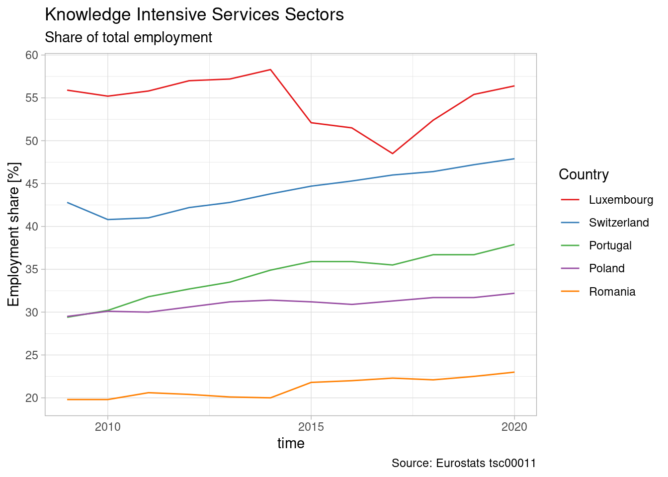
[37] "ME"        "MK"

There are many countries in the dataset which would make a timeseries analysis difficult to read. Sometimes we use dynamic plots or provide filtering to the readers to overcome this but here we’re only looking for a simple static plot. We therefore filter out a few countries. Our choice aimed at having the extremes - Romania and Luxembourg - plus a couple of countries in between.

We also can see that there are statistics for two indicators: Manufacturing jobs and Knowledge Intensive jobs. We’re interested in the later which we use for filtering the data:

country_list <- c("PT", "LU", "CH", "PL", "RO")

data_short <- data_raw %>%
    filter(geo %in% country_list) %>%
    filter(nace_r2 == "KIS")

The eurostats R package provides a labelling function which is very usefull.

data_short_labelled <- label_eurostat(
    data_short, 
    #custom_dic = c(DE = "Germany"), 
    lang = "en") %>%
    mutate(geo = fct_relevel(
        geo, c("Luxembourg", "Switzerland", "Portugal", "Poland", "Romania")))

write_rds(data_short_labelled, here("./posts/20220212/data/tsc00011_data_short_labelled.rds"))

data_short_labelled <- read_rds(here("posts/20220212/data/tsc00011_data_short_labelled.rds"))

Plot

With the data cleaned and sorted, we’re now in a position to produce a plot. We can see strong heterogeniety, ranging from a max at more than 55% for Luxembourg and a min at less than 25% for Romania.

data_short_labelled %>%
    mutate(geo = fct_relevel(geo, c("Luxembourg", "Switzerland", "Portugal", "Poland", "Romania"))) |> 
    ggplot(aes(x = time, y = values, color = geo)) +
    geom_line() +
    scale_y_continuous(n.breaks = 10, name = "Employment share [%]" ) +
    scale_color_brewer(palette = "Set1", name = "Country") +
    theme_light() +
    #theme(legend.position = "bottom") +
    labs(
        title = "Knowledge Intensive Services Sectors",
        subtitle = "Share of total employment",
        caption = "Source: Eurostats tsc00011"
    )

gdp per capita 2022

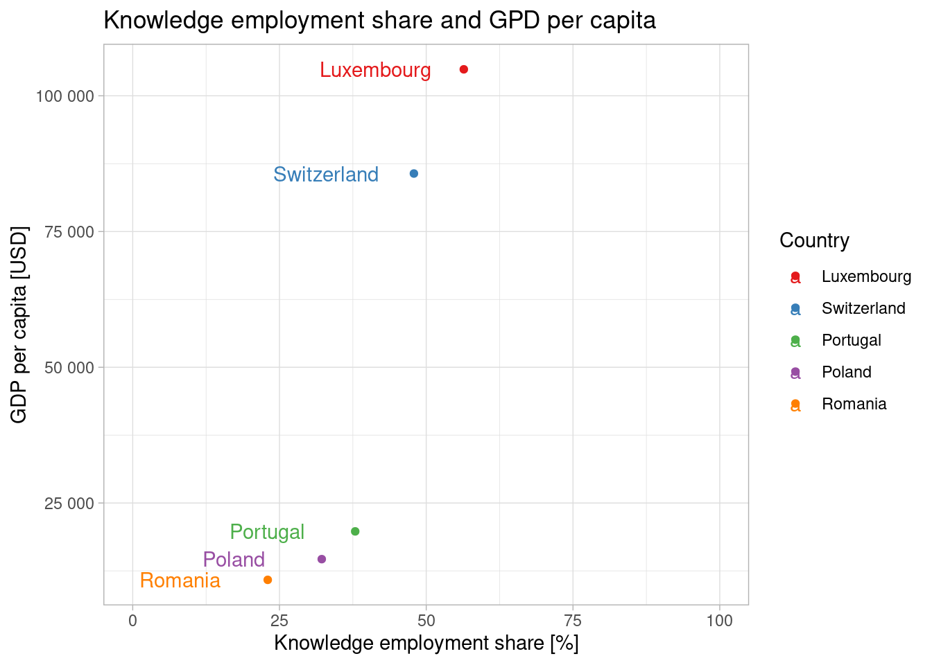
gdp_usdpercapita_2021 <- tribble(
  ~geo, ~gdp_usdpercapita,
  "Switzerland", 85685,
  "Luxembourg", 104879,
  "Portugal", 19772, 
  "Poland", 14661,
  "Romania", 10845
)

data_cor_2021 <- data_short_labelled |> 
  filter(time == "2020-01-01") |> 
  select(geo, employment_share = values) |> 
  left_join(gdp_usdpercapita_2021)

Joining, by = "geo"

data_cor_2021 |> 
  mutate(geo = fct_relevel(geo, c("Luxembourg", "Switzerland", "Portugal", "Poland", "Romania"))) |> 
  ggplot(aes(employment_share, gdp_usdpercapita, color = geo)) +
  geom_point() +
  geom_text(aes(label = geo), nudge_x = -15) +
  coord_cartesian(xlim = c(0, 100)) +
  scale_y_continuous(labels = scales::label_number()) +
  scale_color_brewer(palette = "Set1", name = "Country") +
  labs(
    title = "Knowledge employment share and GPD per capita",
    y = "GDP per capita [USD]",
    x = "Knowledge employment share [%]"
  ) +
  theme_light()