library(tidyverse)
library(tidymodels)
library(rpart.plot)
library(patchwork)
tidymodels_prefer()Machine Learning with R-tidymodels: model tuning
machine learning
Last week I shared some more examples on Classification Models based on the Rbootcamp workshops. Here we continue our summary now with model tuning. The example shown here now covers the full pipeline presented at the workshop including resampling and tuning and can be used as a first basis for application in real life cases.
setup
ridge regression
sample
airbnb <- read_csv(file = "data/airbnb.csv")Rows: 1191 Columns: 23
── Column specification ────────────────────────────────────────────────────────
Delimiter: ","
chr (8): district, host_respons_time, kitchen, tv, coffe_machine, dishwashe...
dbl (14): price, accommodates, bedrooms, bathrooms, cleaning_fee, availabili...
lgl (1): host_superhost
ℹ Use `spec()` to retrieve the full column specification for this data.
ℹ Specify the column types or set `show_col_types = FALSE` to quiet this message.set.seed(123)
airbnb_split <- initial_split(airbnb, prop = 0.75)
airbnb_train <- training(airbnb_split)
airbnb_folds <- vfold_cv(airbnb_train, v = 10)
airbnb_test <- testing(airbnb_split)
doParallel::registerDoParallel()recipe
ridge_recipe <- recipe(
  formula = price ~ .,
  airbnb_train
  ) %>%
  step_dummy(all_nominal_predictors()) %>%
  step_normalize(all_numeric_predictors())
Normalization applies well in regularized regression because the coefficients are scale dependent. Nevertheless there are also there interpretation concerns since standardizing helps comparison but makes interpretation more difficult.
model
ridge_model <-
  linear_reg(mixture = 0, penalty = tune()) %>%
  set_engine("glmnet") %>%
  set_mode("regression")
workflow
ridge_workflow <-
  workflow() %>%
  add_recipe(ridge_recipe) %>%
  add_model(ridge_model)
tune
penalty_grid <- grid_regular(penalty(), levels = 50)ridge_grid <-
ridge_workflow %>%
tune_grid(resamples = airbnb_folds,
grid = penalty_grid)collect_metrics(ridge_grid)# A tibble: 100 × 7
penalty .metric .estimator mean n std_err .config
<dbl> <chr> <chr> <dbl> <int> <dbl> <chr>
1 1 e-10 rmse standard 64.4 10 18.9 Preprocessor1_Model01
2 1 e-10 rsq standard 0.542 10 0.0425 Preprocessor1_Model01
3 1.60e-10 rmse standard 64.4 10 18.9 Preprocessor1_Model02
4 1.60e-10 rsq standard 0.542 10 0.0425 Preprocessor1_Model02
5 2.56e-10 rmse standard 64.4 10 18.9 Preprocessor1_Model03
6 2.56e-10 rsq standard 0.542 10 0.0425 Preprocessor1_Model03
7 4.09e-10 rmse standard 64.4 10 18.9 Preprocessor1_Model04
8 4.09e-10 rsq standard 0.542 10 0.0425 Preprocessor1_Model04
9 6.55e-10 rmse standard 64.4 10 18.9 Preprocessor1_Model05
10 6.55e-10 rsq standard 0.542 10 0.0425 Preprocessor1_Model05
# … with 90 more rowsridge_grid %>%
collect_metrics() %>%
ggplot(aes(penalty, mean, color = .metric)) +
geom_line(size = 1.5) +
facet_wrap(~.metric, scales = "free", nrow = 2) +
theme(legend.position = "none")
(re-tune)
penalty_grid <- tibble(penalty = seq(0, 250, length.out = 200))ridge_grid <-
ridge_workflow %>%
tune_grid(resamples = airbnb_folds,
grid = penalty_grid)collect_metrics(ridge_grid)# A tibble: 400 × 7
penalty .metric .estimator mean n std_err .config
<dbl> <chr> <chr> <dbl> <int> <dbl> <chr>
1 0 rmse standard 64.4 10 18.9 Preprocessor1_Model001
2 0 rsq standard 0.542 10 0.0425 Preprocessor1_Model001
3 1.26 rmse standard 64.4 10 18.9 Preprocessor1_Model002
4 1.26 rsq standard 0.542 10 0.0425 Preprocessor1_Model002
5 2.51 rmse standard 64.4 10 18.9 Preprocessor1_Model003
6 2.51 rsq standard 0.542 10 0.0425 Preprocessor1_Model003
7 3.77 rmse standard 64.4 10 18.9 Preprocessor1_Model004
8 3.77 rsq standard 0.542 10 0.0425 Preprocessor1_Model004
9 5.03 rmse standard 64.4 10 18.9 Preprocessor1_Model005
10 5.03 rsq standard 0.542 10 0.0426 Preprocessor1_Model005
# … with 390 more rowsridge_grid %>%
collect_metrics() %>%
ggplot(aes(penalty, mean, color = .metric)) +
geom_line(size = 1.5) +
facet_wrap(~.metric, scales = "free", nrow = 2) +
theme(legend.position = "none") +
labs(
title = "Model performance vs penalty"
) +
theme_light()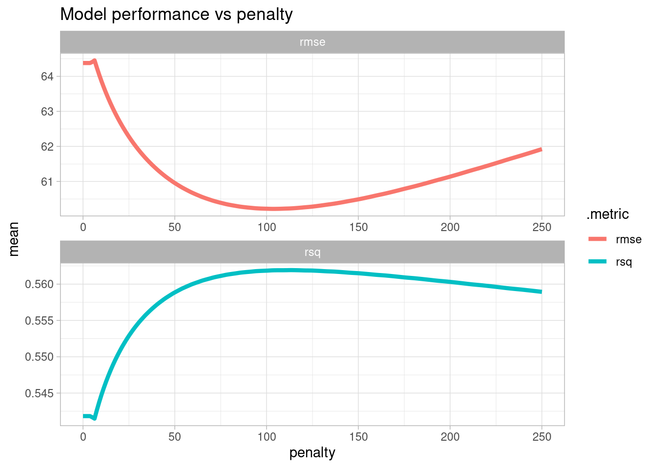
best_ridge <- select_best(ridge_grid, "rmse")final_ridge <-
ridge_workflow %>%
finalize_workflow(best_ridge)fit
ridge_res <- fit(final_ridge, airbnb_train)

tidy(ridge_res)
# A tibble: 35 × 3
term estimate penalty
<chr> <dbl> <dbl>
1 (Intercept) 69.7 103.
2 accommodates 20.9 103.
3 bedrooms 14.0 103.
4 bathrooms 8.58 103.
5 cleaning_fee 0.791 103.
6 availability_90_days 0.820 103.
7 host_response_rate -0.197 103.
8 host_superhost 6.09 103.
9 host_listings_count 2.68 103.
10 review_scores_accuracy 1.79 103.
# … with 25 more rowsridge_res_last <- last_fit(final_ridge, airbnb_split)collect_metrics(ridge_res_last)# A tibble: 2 × 4
.metric .estimator .estimate .config
<chr> <chr> <dbl> <chr>
1 rmse standard 34.1 Preprocessor1_Model1
2 rsq standard 0.417 Preprocessor1_Model1predict
ridge_predict_train <-
  ridge_res %>%
  predict(new_data = airbnb_train) %>%
  bind_cols(airbnb_train %>% select(price))
  # metrics(truth = price, estimate = .pred)
ridge_predict_test <-
ridge_res %>%
predict(new_data = airbnb_test) %>%
bind_cols(airbnb_test %>% select(price))
# metrics(truth = price, estimate = .pred)ridge_predict_train# A tibble: 893 × 2
.pred price
<dbl> <dbl>
1 53.8 58
2 58.0 37
3 115. 170
4 121. 80
5 58.8 30
6 74.1 99
7 66.8 40
8 99.6 92
9 35.1 75
10 62.3 50
# … with 883 more rowsridge_predict_test# A tibble: 298 × 2
.pred price
<dbl> <dbl>
1 96.6 99
2 58.3 50
3 59.1 30
4 28.6 32
5 84.5 85
6 96.9 150
7 56.7 45
8 99.0 45
9 78.7 45
10 120. 230
# … with 288 more rowsmetrics
metrics_ridge_train <- ridge_predict_train %>%
  metrics(truth = price, estimate = .pred)
metrics_ridge_test <- ridge_predict_test %>%
metrics(truth = price, estimate = .pred)metrics_ridge_train# A tibble: 3 × 3
.metric .estimator .estimate
<chr> <chr> <dbl>
1 rmse standard 83.0
2 rsq standard 0.367
3 mae standard 26.8 metrics_ridge_test# A tibble: 3 × 3
.metric .estimator .estimate
<chr> <chr> <dbl>
1 rmse standard 34.1
2 rsq standard 0.417
3 mae standard 24.3 plot
create_model_plot <- function(prediction_data, model_metrics, title_text) {
  annotation_data <- tibble(
    x_position = 100,
    y_position = c(400, 450, 500),
    label_value = str_glue_data(model_metrics, "{.metric}: {round(.estimate, 2)}")
  )

  prediction_data %>%
    ggplot(aes(x = .pred, y = price)) +
    geom_abline(lty = 2) +
    geom_point(alpha = 0.5) +
    geom_text(
      data = annotation_data,
      mapping = aes(x = x_position, y = y_position, label = label_value),
      size = 3
    ) +
    labs(
      title = as.character(title_text),
      caption = "Line = perfect performance",
      x = "Predicted Prices in $",
      y = "True Prices in $"
    ) +
    coord_obs_pred(ratio = 1) + # Scale and size the x- and y-axis uniformly:
    coord_cartesian(x = c(0, 500), y = c(0, 500)) +
    theme_light()
} create_model_plot(ridge_predict_test, metrics_ridge_test, "Ridge Regression")Coordinate system already present. Adding new coordinate system, which will replace the existing one.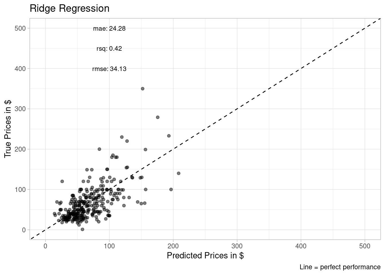
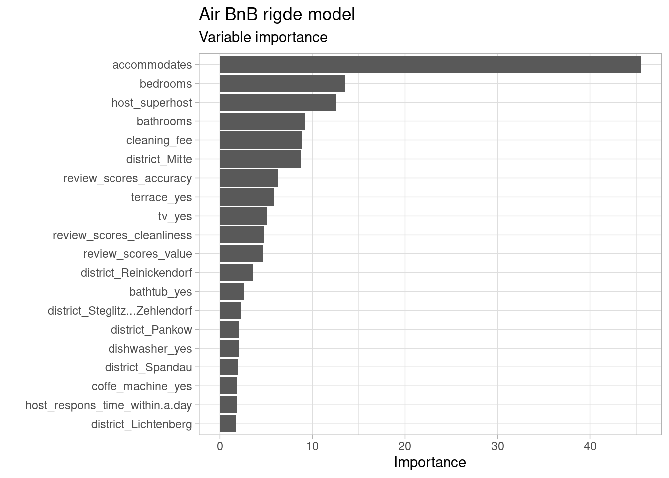
variable importance
library(vip)ridge_res_last %>%
extract_fit_parsnip() %>%
vip(num_features = 20) +
labs(
title = "Air BnB rigde model",
subtitle = "Variable importance"
) +
theme_light()